
Most computers can execute operations in parallel due to their multicore infrastructure. Performing more than one operation simultaneously has the potential to speed up most tasks and has many practical uses within the field of data science. SAS Viya offers several products that facilitate parallel task execution. Many of these tools rely on the asynchronous action execution framework provided by the SAS Viya Cloud Analytic Services (CAS). Others rely on distributing calculations to individual worker nodes. Within CAS, there are tools that handle parallel execution automatically for you, as most CAS actions employ some form of parallel processing. But there are also tools that allow you to write your own parallel task execution frameworks. Here we discuss the benefits of performing parallel task execution and the tools provided in SAS Viya for that purpose.
Use-cases for parallel processing in data science
To explain the usefulness of parallelization in data science, consider the following machine-learning pipeline built using Model Studio.
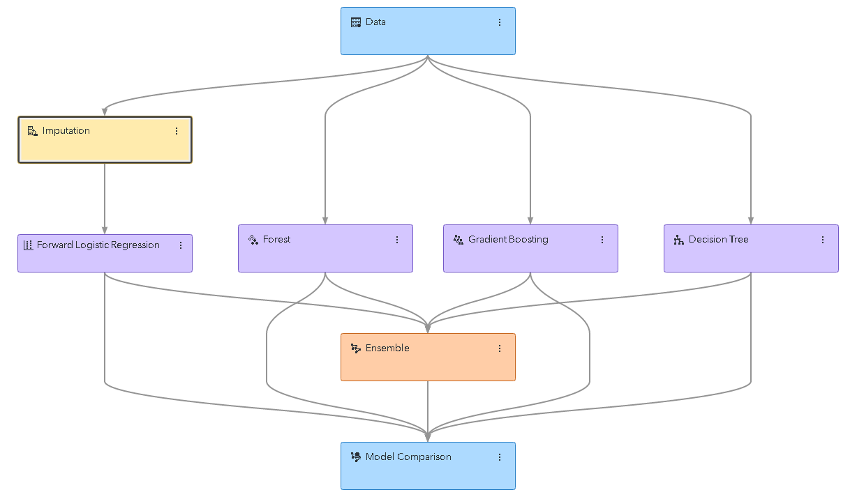
This is a relatively standard modeling pipeline. There are several different modeling nodes, some with preprocessing steps and some without. To train the entire pipeline, each node needs to be trained individually, but some of the nodes depend on other nodes.
For instance, the forward logistic regression node depends on the imputation node, and the ensemble node depends on all the model nodes. But the nodes don’t have to be processed one at a time, there are several nodes that share a common dependency. Take the decision-tree-based nodes, for instance. Each of these nodes only depends on the data node. Once the data node has completed, each of these nodes is free to start training.
If the machine-learning system being used to execute the pipeline (in this case, the CAS server) has sufficient computing resources, it can train all these models at once. Model Studio does just this, executing multiple nodes simultaneously if the nodes do not depend on one another.
Parallel processing within data science is not limited to pipeline training. Many individual algorithms or steps themselves have parallel implementations. A forest model, for instance, requires training many individual trees that are then ensembled. Unlike in a gradient boosting model, these trees do not depend upon one another. Due to their independence, these trees can be trained in parallel, and many algorithms do just that. The forests in SAS Viya seek to gain as many performance improvements as possible using parallelization methods, as do most other CAS actions.
Additionally, many operations performed on data can be parallelized to an extreme degree. In model scoring, a model typically only needs information from a single observation to produce a scored value, so each observation is free to be scored simultaneously. Models in CAS do this, scoring as many rows at one time as they can physically handle. This sort of parallelism is not limited to scoring, and many data-level operations can be parallelized in this way.
Where parallelism is done for you
As demonstrated above with random forests and the Model Studio pipeline, many analytic algorithms have room in their design to accommodate parallelism. However, implementing parallel algorithms is typically more difficult than their sequential counterpart.
Fortunately, most of the products included in SAS Viya do this work for you. Products like Model Studio can handle connections from many users simultaneously so they can work concurrently without interrupting one another. The CAS server itself also works to parallelize tasks, and like Model Studio can handle connections from multiple users at once. Additionally, the actions being submitted by users to CAS further parallelize tasks by taking advantage of CAS’s multi-node, multithreaded architecture.
Further utilizing parallelism in CAS
For users that are familiar with the programming interfaces to SAS Viya, there are ways to take further advantage of CAS’s parallelization capabilities. There are several interfaces through which parallel task execution is possible, including CAS DATA Step, optimization actions such as solveBlackBox or autotuning, the IML action, parallel CAS sessions, and many others.
The following sections will each provide a simple example of parallel task execution using one of these tools. In these examples. the CAS server being used has five workers. When using these tools, you should take care not to put too much load on the CAS server so that the performance of other users’ sessions is not hindered.
The autotuning action documentation has a section titled “Determining the Number of Parallel Evaluations” which goes into detail about determining an appropriate number of parallel tasks to execute at once. The concepts described there are shared by many other CAS actions and are applicable to the actions in the examples below.
CAS DATA step
Data stored in CAS is typically distributed amongst all the workers and threads in the cluster, and when CAS DATA Step processes this distributed data it typically does so in parallel, each thread independently processing some portion of the rows associated with that worker. This is the default behavior of the CAS DATA step and a user must specify the single=YES option to process data one row at a time. But for the sake of demonstration, the following code will compare the processing duration for a simple DATA step program that scores a logistic regression model using both the single=YES and single=NO options.
/* Example Data, 100x Replicates */ data sascas1.HMEQ; set sampsio.HMEQ; do i = 1 to 100; output; end; drop I; run; proc cas; /* Load Actionset */ loadactionset "datastep"; /* Define datastep code as a string */ source ds_code; data hmeq_scored; set hmeq; /* Score linear model */ linp = 0.9474; linp = linp + 0.000022 * loan; linp = linp + -3.58E-7 * loan; linp = linp + 2.431E-6 * loan; exp_linp = exp(linp); P_BAD1 = exp_linp / (exp_linp + 1); drop linp exp_linp; run; endsource; /* run data step in single thread */ start_time = datetime(); datastep.runCode / code = ds_code, single = "YES"; single_time = datetime() - start_time; /* run data step in multiple threads on multiple workers */ start_time = datetime(); datastep.runCode / code = ds_code; threaded_time = datetime() - start_time; print "Performance gain with single='NO': " single_time / threaded_time; quit; |
CAS DATA Step Example, CAS Server with 5 workers, 3.5x speedup
The example DATA step above is 3.5x faster when you allow the DATA step to process the rows in a distributed manner. This is not always possible when there is a row-order dependency that must be obeyed in the DATA step code. But for DATA step code that only affects one row at a time, this is a very powerful method.
Optimization/Autotuning actions
SAS Viya offers a wide range of autotuning actions and optimization routines through different action interfaces. Optimization oftentimes involves evaluating some metric given a set of parameters. In the case of autotuning, the metric is model accuracy and the parameters are the model’s hyperparameters. The evaluation of a single set of hyperparameters is unaffected by the value of another set of hyperparameters, much in the same way as the machine learning models in the pipeline described earlier do not affect one another. Thus, the autotuning actions in SAS Viya allow models to be submitted in parallel when evaluations are performed. A machine learning model is typically a high-load task for a CAS server. So the number of parallel models submitted simultaneously should be throttled or performance will suffer. The following code demonstrates the power of evaluating multiple model hyperparameter combinations simultaneously.
/* Send data to CAS */ data sascas1.hmeq; set sampsio.hmeq; run; proc cas; /* store tuning parameters in a dictionary */ tune_parameters = { trainOptions={ table = "HMEQ" target="BAD", inputs={ "CLAGE", "CLNO", "DEBTINC", "LOAN", "MORTDUE", "VALUE","YOJ", "DELINQ", "DEROG", "JOB", "NINQ" }, nominals={"DELINQ", "DEROG", "JOB", "NINQ", "BAD"} } }; /* train/score models sequentially */ start_time = datetime(); autotune.tuneForest / tune_parameters + {tunerOptions={seed=54321, nParallel=1}}; single_time = datetime() - start_time; /* train/score models in parallel */ start_time = datetime(); autotune.tuneForest / tune_parameters + {tunerOptions={seed=54321, nParallel=10}}; parallel_time = datetime() - start_time; print "Performance gain with more threads: " single_time / parallel_time; quit; |
Autotuning Example, CAS Server with 5 workers, 2.6x speedup
Adjusting the number of parallel model evaluations had a massive impact on the total autotuning duration, finishing 2.6x quicker than the sequential implementation.
SAS IML
PROC IML is an exceptionally powerful tool available for SAS users. The same can be said for the IML action set within SAS Viya. Much of the functionality available in the IML procedure is also available in the action. Several new features have been added to take advantage of CAS’s distributed computing capabilities. The following program is a simple example of taking the group-wise mean of a column. First, the group means are computed using traditional IML methods. Then a new IML action function, MapReduceTable, is employed on the same task.
/* Example Data, 100x Replicates */ data sascas1.hmeq; set sampsio.hmeq; do i = 1 to 100; output; end; drop I; run; proc cas; /* create iml code as a string */ source iml_code; /* time sequential group-means calculation */ start_time = time(); /* read CAS table into IML */ hmeq = tableCreateFromCAS("","hmeq"); jobs = tableGetVarData(hmeq,"JOB"); if any(missing(jobs)) then jobs[loc(missing(jobs))] = "_miss_"; loan = tableGetVarData(hmeq,"loan"); /* sort, create index */ jobs_index = j(1,nrow(jobs),.); call sortndx(jobs_index,jobs,1); jobs = jobs[jobs_index]; loan = loan[jobs_index]; B = uniqueBy(jobs,1) // (nrow(jobs) + 1); /* allocate result matrices */ job_levels = j(1,nrow(B) - 1,jobs[1]); job_loan_avg = j(1,nrow(B) - 1,.); /* calculate group-wise mean */ do i = 1 to nrow(B) - 1; job_levels[i] = jobs[B[i]]; job_loan_avg[i] = mean(loan[B[i]:(B[i+1]-1)]); end; /* summarize sequential run */ single_duration = time() - start_time; print job_levels, job_loan_avg; print "Standard Duration: " single_duration; /* time map-reduce group-mean calculation */ start_time = time(); start groupMeanMap(params,x_in,c_in,groupSummary); /* collect partial sums for data on worker nodes */ /* x_in,c_in contain numeric/character variable data */ jobs = c_in; if any(missing(jobs)) then jobs[loc(missing(jobs))] = "_miss_"; loan = x_in; /* sort, create index */ jobs_index = j(1,nrow(jobs),.); call sortndx(jobs_index,jobs,1); jobs = jobs[jobs_index]; loan = loan[jobs_index]; B = uniqueBy(jobs,1) // (nrow(jobs) + 1); /* store partial sums in a list */ groupSummary = []; /* calculate mean by group */ do i = 1 to nrow(B) - 1; /* summary statistics for group */ sum = sum(loan[B[i]:(B[i+1]-1)]); count = sum(^missing(loan[B[i]:(B[i+1]-1)])); if count > 0 then mean = sum / count; else mean = .; /* append stats to list */ call listAddItem( groupSummary, [ #sum = sum, #count = count, #mean = mean ] ); call listSetName(groupSummary,listLen(groupSummary),jobs[B[i]]); end; return 0; finish; start groupMeanRed(groupSummary,groupSummaryPart); /* combine partial sums */ /* add counts and sum, divide */ if isEmpty(groupSummary) then do; groupSummary = groupSummaryPart; end; else do; /* not all partial sums will contain all groups */ /* check which groups are in the summary lists */ new_levels = listGetAllNames(groupSummaryPart); old_levels = listGetAllNames(groupSummary); do i = 1 to ncol(new_levels); /* combining sums/counts */ if any(old_levels = new_levels[i]) then do; /* combine stats */ sum = groupSummary$(new_levels[i])$"sum" + groupSummaryPart$(new_levels[i])$"sum"; count = groupSummary$(new_levels[i])$"count" + groupSummaryPart$(new_levels[i])$"count"; if count > 0 then mean = sum / count; else mean = .; /* overwrite existing summary data */ groupSummary$(new_levels[i]) = [ #sum = sum, #count = count, #mean = mean ]; end; else do; /* add new group */ call listAddItem(groupSummary,groupSummaryPart$(new_levels[i])); call listSetName(groupSummary,listLen(groupSummary),new_levels[i]); end; end; end; return 0; finish; /* call mapper/reducer functions */ groupMeans = mapReduceTable( {"groupMeanMap","groupMeanRed"}, ., "JOB" || "LOAN", "hmeq", 10000 ); /* process return from mapReduce */ job_levels = listGetAllNames(groupMeans); job_loan_avg = j(1,ncol(job_levels),.); do i = 1 to ncol(job_levels); job_loan_avg[i] = groupMeans$(job_levels[i])$"mean"; end; parallel_duration = time() - start_time; /* summarize results */ print job_levels, job_loan_avg; print "Map Reduce Duration: " parallel_duration; print "Gain from Map Reduce: " (single_duration / parallel_duration); endsource; /* call iml action */ loadactionset "iml"; iml.iml / code = iml_code; quit; |
IML Action Example, CAS Server with 5 workers, 9.9x speedup
For this problem, the MapReduceTable function completed 9.9x faster than the traditional IML implementation. MapReduceTable takes advantage of the fact that the data set is distributed amongst the CAS worker nodes. Each worker/thread can compute the partial sums for the rows available to it. The result is a much faster implementation of the group mean algorithm. This trivial example only scratches the surface of what is possible in the IML action. Please consult the SAS IML documentation for more details. Consider reading The DO Loop which is full of tips for SAS/IML users.
Parallel CAS sessions
Users can interact with the CAS server indirectly using a product such as SAS Visual Analytics or Model Studio. Users can also interact with the CAS server using programming languages such as Python and R. First you establish a CAS session, then submit actions to that session for processing. The CAS session will then process your actions one at a time. But you’re not limited to just one CAS session, you can start as many sessions as you’d like. You can then send actions to each of these sessions individually. Each session will work to process the actions in its own action queue. The result is that the actions you’ve submitted will be processed more than one at a time, in parallel. The example program below trains two forest models. First, the models are trained sequentially, then in parallel, and their performance is compared.
data sascas1.HMEQ(promote="YES"); /* Promote to make available to other sessions */ set sampsio.HMEQ; run; proc cas; source casl_code; /* Mini-Reference: 1. create_parallel_session() - function to start a parallel session, returns session name as string 2. term_parallel_session(session) - function to end a parallel session, accepts session name as string 3. wait_for_next_action() - waits for action to complete in a parallel session, returns dictionary with results, status, session, and job information 4. action session="" option - specifies which session will run action. 5. action async="" option - gives a job name to an asynchronous action, returns as part of the return from wait_for_next_action() */ /* Load Actionset, Save Forest Parameters */ loadActionset "decisionTree"; forest_parameters = { table = "HMEQ" target="BAD", inputs={ "CLAGE", "CLNO", "DEBTINC", "LOAN", "MORTDUE", "VALUE","YOJ", "DELINQ", "DEROG", "JOB", "NINQ" }, nominals={"DELINQ", "DEROG", "JOB", "NINQ", "BAD"}, nTrees = 1000 }; /* Call Actions Sequentially */ start_time = datetime(); decisionTree.forestTrain result=forest_res status=forest_st / forest_parameters; decisionTree.forestTrain result=forest_res2 status=forest_st2 / forest_parameters; sequential_time = datetime() - start_time; /* Inspect Results */ print "Duration of sequential calls: " sequential_time; title "First Forest Model Results"; print forest_res; title "Second Forest Model Results"; print forest_res2; title; /* Call Actions in Parallel */ start_time = datetime(); /* Start Parallel Sessions */ num_sessions = 2; sessions = {}; results = {}; do i = 1 to 2; sessions[i] = create_parallel_session(); end; /* Submit Sessions */ decisionTree.forestTrain session = sessions[1] async = "first_forest" / forest_parameters; decisionTree.forestTrain session = sessions[2] async = "second_forest" / forest_parameters; /* Wait for Sessions to return */ job = wait_for_next_action(); do while(job); results[job["job"]] = job; job = wait_for_next_action(); end; /* Terminate Sessions */ do session over sessions; term_parallel_session(session); end; parallel_time = datetime() - start_time; /* Inspect Results */ print "Duration of parallel calls: " parallel_time; title "First Forest Model Results, Parallel Call"; print results["first_forest"]["result"]; title "Second Forest Model Results, Parallel Call"; print results["second_forest"]["result"]; title; /* Print Results */ print "Speed Increase from Parallel Sessions: " sequential_time / parallel_time; endsource; loadActionset "sccasl"; sccasl.runCasl / code = casl_code; quit; |
Parallel Session Example, CAS Server with 5 workers, 1.5x speedup
When the above code is executed, the actions submitted to multiple sessions complete 1.5x faster than the actions submitted to a single session. The exact speedup is dependent on the SAS Viya installation and the actions themselves. But it is not uncommon to find scenarios where this multi-session paradigm can reduce the total amount of time it takes a series of actions to complete.
Conclusion
As demonstrated above, the parallel processing features in CAS can greatly improve the performance of many common data science algorithms. Not all tasks can be parallelized, and the performance gains may not always be as great as the ones shown here, but hopefully, this has given you some ideas for your next project.
The next post in this series will focus on submitting actions in parallel from CASL. It will give a few best practices for handling parallel action executions. It will also show a few examples where the practice greatly improves performance.
LEARN MORE | SAS YIYAWANT MORE GREAT INSIGHTS MONTHLY? | SUBSCRIBE TO THE SAS LEARNING REPORT

1 Comment
Pingback: Tips for parallel processing in CASL - The SAS Data Science Blog